Editor’s note: We are delighted to announce a new paper by Swedish mathematician Ola Hössjer and Discovery Institute Senior Fellow Ann Gauger in the journal BIO-Complexity. The new research describes scientific work demonstrating that it is possible for the human species to have originated with a pair rather than thousands of individuals. What follows is the first of two posts by Ann describing the work in detail.
If you asked pretty much any population geneticist about human origins they would say, “All the evidence says the effective population size has never been below several thousand.” That’s certainly what Dennis Venema thought, and said most emphatically in the book Adam and the Genome:
The sun is at the center of our solar system, humans evolved, and we evolved as a population.
Put most simply, DNA evidence indicates that humans descend from a large population because we, as a species, are so genetically diverse in the present day that a large ancestral population is needed to transmit that diversity to us. To date, every genetic analysis estimating ancestral population sizes has agreed that we descend from a population of thousands, not a single ancestral couple. (p. 55)
He was also quite dismissive of those of us who were working on the problem from a different perspective.
[T]here does not appear to be anyone in the antievolutionary camp at present with the necessary training to properly understand the evidence, much less offer a compelling case against it. (Adam and the Genome, p. 65)
I suppose Venema can be excused for that statement though he should have been less dismissive. Venema might be excused for saying I wasn’t qualified. But I knew how to find someone who was. Ola Hössjer of Stockholm University Mathematics Department knows population genetics as well or better than Dennis, and applied mathematics better than that.
Teaming Up
When I first met Ola at a meeting in Copenhagen, we discussed the outlines of what would become the model whose results we report today. The key to addressing the question of our possible origin from two was to model the question directly: start with a population of two and go forward, while keeping track of genetic diversity, to see if we could duplicate the diversity we see in the human population today. The difficulty was that this kind of forward modeling is extremely memory intensive and all but the largest computers cannot go very many generations into the future. Besides that difficulty, I gave him a long list of variables the model should incorporate, an impossible list, I thought.
Time passed, and then I had occasion to check in with Ola again. He had a model we now call Haplo that contained within it a simple but brilliant idea. He would start first from current data and use a method called standard coalescence to trace the lineages backward in time, like growing a forest from stems to branches to trunks. Then once he had that forest of trunks, he pruned the picture of all non-productive branches, those that did not have any progeny in the future, the “dead ends,” and used it as a framework for a new forward-looking model. The pruning saved considerable memory and reduced the computational load. This meant we could go deeper in time or handle larger populations. See the figure below.
Each row represents a generation, with the present at the bottom, and each ball is a chromosome. The colored dots are different mutations or Single Nucleotide Polymorphisms (SNPs) the chromosome carries. The links from generation to generation show the ancestral lineage of each chromosome going back in time.
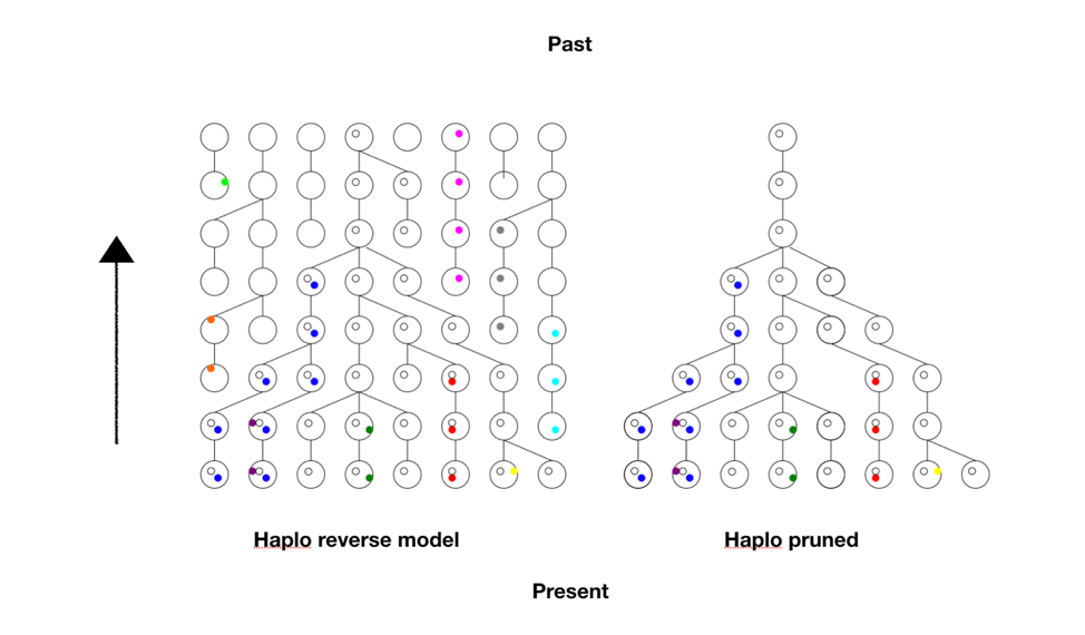
First the tree (or forest) in reverse is obtained, much larger and complex than this here, and pruned to reveal nothing but the lineages that led to the present. So this provided the framework, the matrix upon which the forward model will run. The computer doesn’t have to keep track of all possible choices at all possible positions. Look at the pruned tree and notice all the spaces the computer doesn’t have to store in memory. It adds greatly to what the program can accomplish.
There is one more step in the model description to consider. We proposed to test whether we could have come from two first parents. The model is based on tracking chromosomes—we each have a double set, one from mom and one from dad. In genetic terms a chromosome set is N, and we are diploid, or 2N, creatures. To model two first parents in terms of chromosomes means there are four sets of chromosomes to start out. We don’t start at 1, or 2, we start at 4 on the coalescence tree. See Figure B below.

There are two ways to arrive at a situation with two individuals as founders of the human race. One is a sudden extreme bottleneck, from a pre-existing population of thousands down to just two. This would result in a restriction to just four chromosomes with heterogeneous SNPs on all four chromosomes, but those four chromosomes could still carry 75% of the previous population’s heterozygosity, provided population growth was good, especially in the beginning. This scenario was actually a favored model of speciation for many years. The idea was that sudden isolation would bring a new combination of genes together and lead to new behaviors or morphologies. If the isolation continued the new traits would potentially become the norm and speciation would be complete. One can imagine this scenario in a world still populated by other hominids, but the pair was isolated in a valley or gorge; one can imagine a scenario more extreme where all hominids except those two were wiped out.
The second way to arrive at a single pair as founders would be by a unique origin, de novo, by means unknown. This situation could either have identical chromosomes, mixed chromosomes, or unique chromosomes.
Now we have to choose the conditions for running the model: the population growth rate, the mutation rate, the time the simulation runs, and any initial conditions.
Our goal was to use as parsimonious a model as possible, to test under a straightforward standard set of assumptions whether it was possible to duplicate current genetic diversity starting from just two individuals.
So we chose population growth curves with an initial doubling time of roughly every 10 generations, until a population of 16,000 was reached, where it held steady. This is a reasonable growth rate, assuming mortality is not high. The mutation rate chosen was smack in the middle of reported rates.
There is one other factor affecting the model’s results, and it’s very important. It has to do with the initial state of the chromosomes. There are multiple ways the four chromosomes could be modeled: all four identical, with no variation at the start, ab initio, 4 distinct chromosomes with each having unique SNPs, or 4 chromosomes with some SNPs shared and some not. Or they could be mixed in blocks. To get an idea of the possibilities, see the figure below. The distribution of initial diversity has a direct bearing on outcomes.

We chose to use the top left scenario with every chromosome unique and no shared SNPs, but other models can be tested in the future. But the other issue is how much! We will return to that question in a bit.
The Fun Begins
We took the data from the 1000 genomes project and generated a standard Allele Frequency Spectrum for the data. This graph is a standard statistical method for displaying genetic diversity in a population. It is going to take some explaining.
Let’s start with what an allele is. An allele in this context is a changed nucleotide at a particular position, so for example, A instead of C in a sequence: AACCGGGATT becomes AAACGGGATTT. The 1000 Genomes Project has kept a record of all the allelic differences in 5008 genomes, or tens of millions of alleles.
Each allele in this graph is biallelic, which means there are only two variants, as above, not three or four. That means that if there are 0.2 A (20%) there will be 0.8 C (80%), since the frequency adds up to 1.0 for each position. After going through all the alleles, the number of alleles at each frequency (%) are graphed. Below are the results for the 1000 Genomes Project.
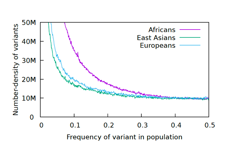
The reason for the upswing to the left on all the curves is that mutations are continually happening, and since they happen one at a time, they are by definition very very rare, with a frequency <<<.01. Most of the time new mutations disappear again without a trace but sometimes they increase in frequency and move to the right in the curve, which is why the curve has the slope it does. The difference between Africans and Asians and Europeans is thought to be because Asians and Europeans went through a bottle when they migrated out of Africa, which reduced their genetic variability (they preferentially lost the rare alleles and have had to rebuild them over time).
One last population statistic to look at: it is called the Linkage Disequilibrium Graph or LD Graph. In brief, it displays a picture of how tightly linked genes are along the chromosome, which has to do with how often chromosomes recombine during meiosis. (Hang on, I’ll explain.) When eggs and sperm are being made, at a certain stage the chromosome pairs come together and line up tightly, zipping together. Then something remarkable called crossing over, or recombination, happens. Somewhere along the arm of the chromosome the chromosomes break and the outer pieces form connections with the opposite inner chromosomes. The result is a shuffling of the DNA into new combinations of alleles.

But other factors can affect linkage as well. Are the interactions between genes that make them necessary in certain combinations or lethal in others? That can serve to keep certain groups of genes tightly coupled. Are there structural reasons why recombination is favored or disfavored in a particular spot? That can also change things.
In any case, there is a particular curve associated with LD. Several different statistics have been developed to describe the distribution of LD along chromosomes, from the centromere, which can be thought of as the center or beginning, to the telomere, the outer edge of the chromosome. In the chromosomes pictured above, the centromeres are constrictions a little more than halfway up. The chromosomes have two arms. Some have only one.
Without further ado, here are the LD graphs for the 1000 Genomes Project.
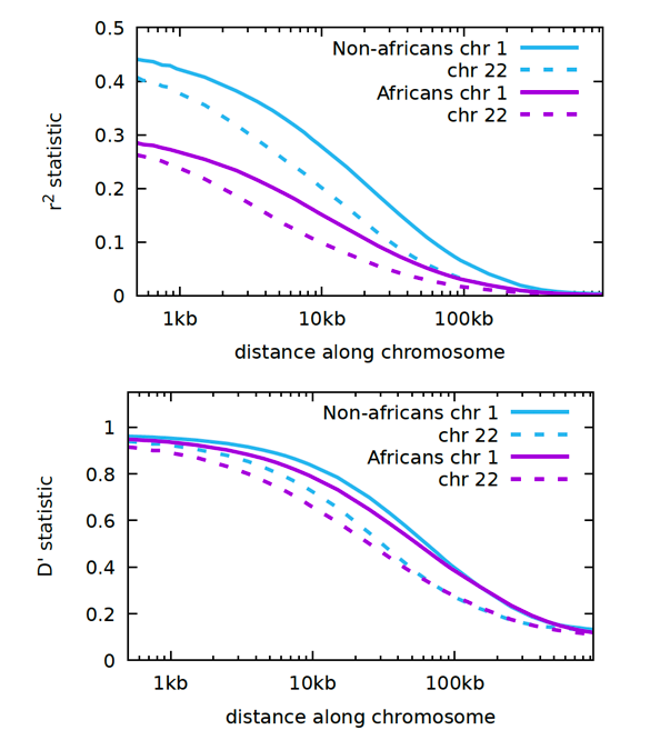
Start high at the centromere and go low the further out you go. This is called an inverse sigmoidal curve. Chromosome 1 is the largest chromosome and chromosome 22 is the smallest.
Now you have the description of the model and the description to the data from the 1000 Genome Project we are trying to match. That is the goal, to find conditions that duplicate the 1000 Genomes curves in a realistic scenario. Oh, and to do it in a parsimonious, minimal way, with as few unusual conditions as possible.
Reminder: The population growth curve is doubling every 10 generations until reaching 16,000, standard mutation rate, initial population 2.
The only other choice is the amount of initial variation on the chromosome. With a bottleneck scenario there would automatically be variation carried over from the population before, in roughly the same amount as the flat part of the AFS curve, where the vast majority of the population’s variation is. So with the single couple origin, when we chose to put in diversity, we chose to put in that same amount of diversity as for the bottlenecked couple. Other values could of course be chosen; we also ran the model with no initial diversity.
So now we come to the moment of the great reveal.


Some things to notice:
Both scenarios have the same conditions: the population starts with 2 doubles every 10 generations until reaching 16,000; 48 mutations per haploid generation, 20 years/generation.
Scenario 1: no primordial diversity Time to match current diversity 2 million years
Scenario 2: with primordial diversity Time to match current diversity 500 thousand years
The Take Home
It is definitely possible for us to have come from a starting point of two. Whether by a bottleneck or by a unique event the numbers say it is possible. 2 million years corresponds to the time of the first hominid to be called Homo, Homo erectus. His exact time and place of origin are unknown but are thought to be in Africa. The 500,000-year mark is near the time of the Neanderthals and Denisovans.
But these numbers are not fixed in stone. They are subject to change: a change in population structure, mortality, mutation rate, birth rate, migration, selection, all can influence the results. The amount of initial diversity, or its distribution, can as well. Changing the population size or time by half can be reversed by multiplying the mutation rate by two. In other words, we have a relationship than can be tweaked and studied, and its parameters can be worked out, but as one of its creators said, the model is “underdetermined.” That’s putting it mildly.
Once again, the precise age of the first couple is not the main point of this study. That there could be a first couple at all is the point.
Image credit: Johannes Plenio via Unsplash.