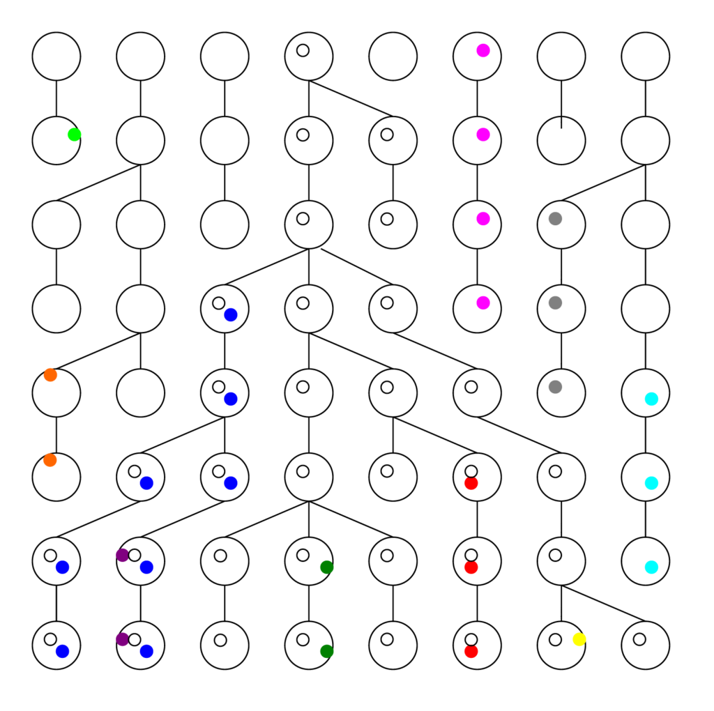
All mutations start as single copy-errors but some of them increase in the population by random processes. Random differences in reproductive success cause some lineages to branch, and others to go extinct. Mutations are presumed to happen randomly at a more-or-less constant rate and accumulate as they are inherited by descendants.
See the figure below. Each row represents a generation, with the present at the bottom, and each ball is a chromosome. The colored dots are different mutations or Single Nucleotide Polymorphisms (SNPs) the chromosome carries. The links from generation to generation show the ancestral lineage of each chromosome going back in time.
Mutation and Genetic Drift
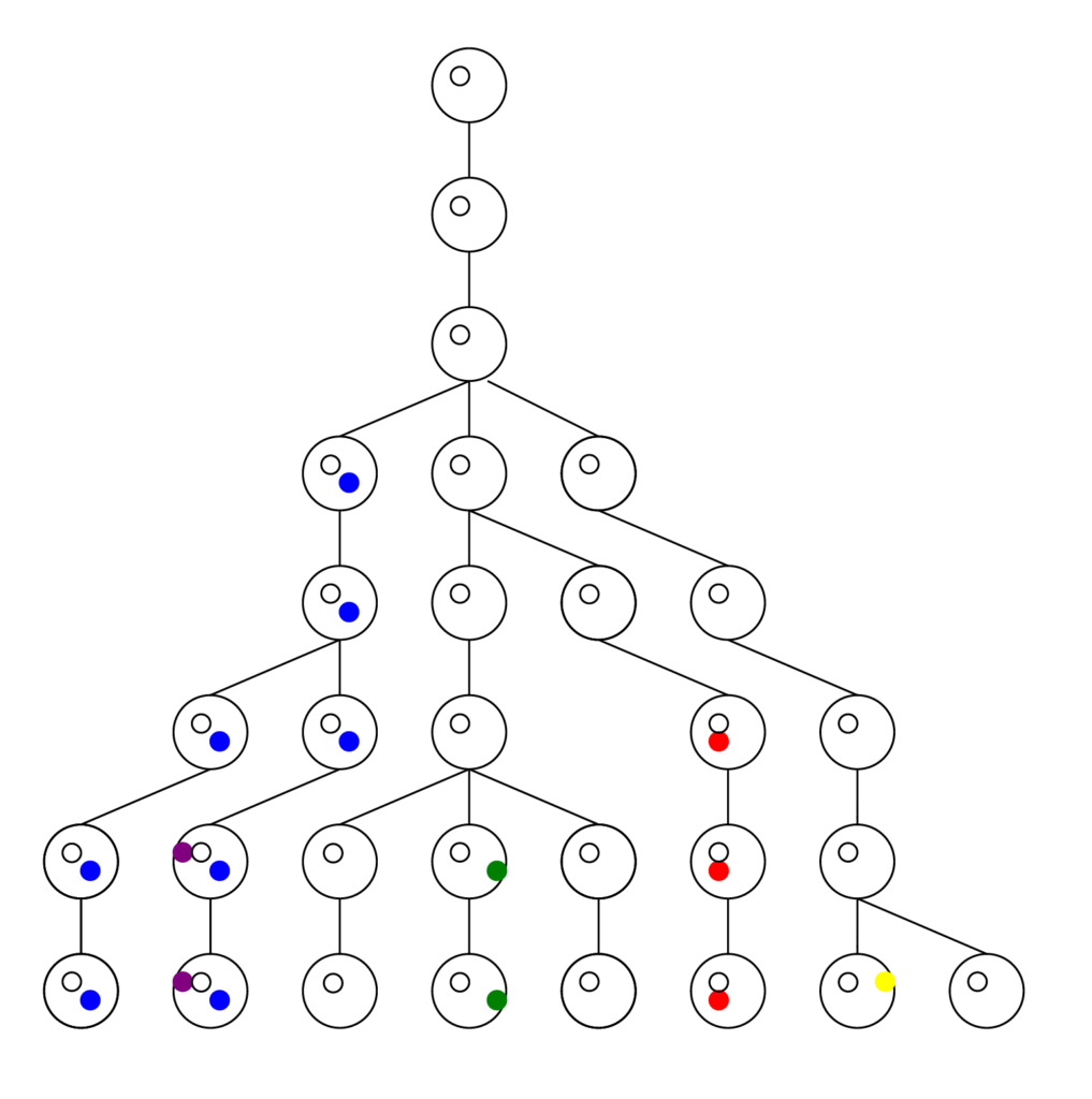
Usually people think of generations as growing forward in time, with twigs coming off branches, and branches off the trunk. Scientists stand in the present and look back in time to try to figure out what happened. Therefore the convention is to count generations backwards in time, where t=0 is the present. The process of lineages branching, when looked at backwards in time, from bottom to top, becomes a process of lineages coalescing. This is an extremely important concept in modern population genetics.
Notice that even in a constant population, the graph diverges from (or converges towards) a single ancestor. Intuitively, this tells us that some of the same results that apply to a constant population also apply to a population that grew from a single ancestor (or a single couple). Thus it is not necessarily easy to tell the difference, which is a crucial point we will discuss later. There are several things worth noting from these figures
- Many mutations go extinct. In a growing population, fewer do. In a shrinking population, more do. We can see only ancestral mutations.
- Ancestral mutations at or before the common ancestor are present in every individual in the final generation. They have been fixed in the population, and are no longer variants.
- There are more recent ancestral mutations, but each has proportionally fewer copies in the final generation (on average).
First the tree (or forest) in reverse is obtained, much larger and complex than this here, and pruned to reveal nothing but the lineages that led to the present. This provides the framework, the matrix upon which the forward model runs. The computer doesn’t have to keep track of all possible choices at all possible positions. Look at the pruned tree and notice all the spaces the computer doesn’t have to store in memory. It adds greatly to what the program can accomplish.
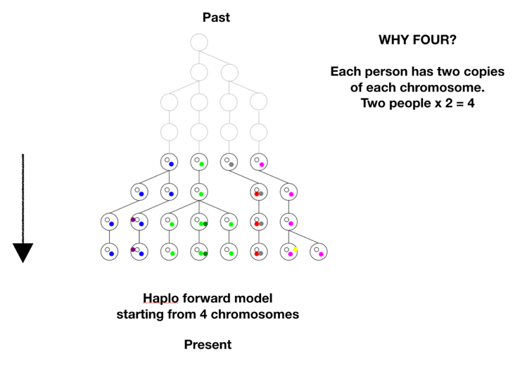
There is one more step in the model description to consider. We proposed to test whether we could have come from two first parents. The model is based on tracking chromosomes—we each have a double set, one from mom and one from dad. In genetic terms a chromosome set is N, and we are diploid, or 2N, creatures. To model two first parents in terms of chromosomes means there are four sets of chromosomes to start out. We don’t start at 1, or 2, we start at 4 on the coalescence tree. See Figure B below.
There are two ways to arrive at a situation with two individuals as founders of the human race. One is a sudden extreme bottleneck, from a pre-existing population of thousands down to just two. This would result in a restriction to just four chromosomes with heterogeneous SNPs on all four chromosomes, but those four chromosomes could still carry 75% of the previous population’s heterozygosity, provided population growth was good, especially in the beginning. This scenario was actually a favored model of speciation for many years. The idea was that sudden isolation would bring a new combination of genes together and lead to new behaviors or morphologies. If the isolation continued the new traits would potentially become the norm and speciation would be complete. One can imagine this scenario in a world still populated by other hominids, but the pair was isolated in a valley or gorge; one can imagine a scenario more extreme where all hominids except those two were wiped out. The second way to arrive at a single pair as founders would be by a unique origin, de novo, by means unknown. This situation could either have identical chromosomes, mixed chromosomes, or unique chromosomes. Now we have to choose the conditions for running the model: the population growth rate, the mutation rate, the time the simulation runs, and any initial conditions. Our goal was to use as parsimonious a model as possible, to test under a straightforward standard set of assumptions whether it was possible to duplicate current genetic diversity starting from just two individuals. So we chose population growth curves with an initial doubling time of roughly every 10 generations, until a population of 16,000 was reached, where it held steady. This is a reasonable growth rate, assuming mortality is not high. The mutation rate chosen was smack in the middle of reported rates. There is one other factor affecting the model’s results, and it’s very important. It has to do with the initial state of the chromosomes. There are multiple ways the four chromosomes could be modeled: all four identical, with no variation at the start, ab initio, 4 distinct chromosomes with each having unique SNPs, or 4 chromosomes with some SNPs shared and some not. Or they could be mixed in blocks. To get an idea of the possibilities, see the figure below. The distribution of initial diversity has a direct bearing on outcomes.
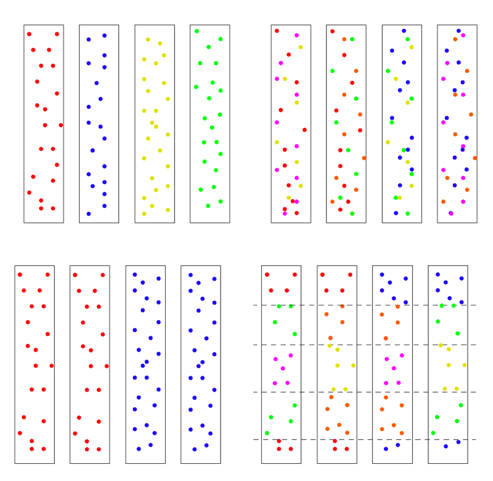
We chose to use the top left scenario with every chromosome unique and no shared SNPs, but other models can be tested in the future. But the other issue is how much variation! We will return to that question in a bit.
The Fun Begins
We took the data from the 1000 genomes project and generated a standard Allele Frequency Spectrum for the data. This graph is a standard statistical method for displaying genetic diversity in a population. It is going to take some explaining. Let’s start with what an allele is. An allele in this context is a changed nucleotide at a particular position, so for example, A instead of C in a sequence: AACCGGGATT becomes AAACGGGATTT. The 1000 Genomes Project has kept a record of all the allelic differences in 5008 genomes, or tens of millions of alleles. Each allele in this graph is biallelic, which means there are only two variants, as above, not three or four. That means that if there are 0.2 A (20%) there will be 0.8 C (80%), since the frequency adds up to 1.0 for each position. After going through all the alleles, the number of alleles at each frequency (%) are graphed. Below are the results for the 1000 Genomes Project.
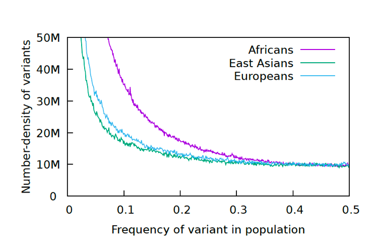
The reason for the upswing to the left on all the curves is that mutations are continually happening, and since they happen one at a time, they are by definition very very rare, with a frequency <<<.01. Most of the time new mutations disappear again without a trace but sometimes they increase in frequency and move to the right in the curve, which is why the curve has the slope it does. The difference between Africans and Asians and Europeans is thought to be because Asians and Europeans went through a bottle when they migrated out of Africa, which reduced their genetic variability (they preferentially lost the rare alleles and have had to rebuild them over time). One last population statistic to look at: it is called the Linkage Disequilibrium Graph or LD Graph. In brief, it displays a picture of how tightly linked genes are along the chromosome, which has to do with how often chromosomes recombine during meiosis. (Hang on, I’ll explain.) When eggs and sperm are being made, at a certain stage the chromosome pairs come together and line up tightly, zipping together. Then something remarkable called crossing over, or recombination, happens. Somewhere along the arm of the chromosome the chromosomes break and the outer pieces form connections with the opposite inner chromosomes. The result is a shuffling of the DNA into new combinations of alleles.
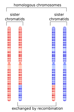
But other factors can affect linkage as well. Are the interactions between genes that make them necessary in certain combinations or lethal in others? That can serve to keep certain groups of genes tightly coupled. Are there structural reasons why recombination is favored or disfavored in a particular spot? That can also change things. In any case, there is a particular curve associated with LD. Several different statistics have been developed to describe the distribution of LD along chromosomes, from the centromere, which can be thought of as the center or beginning, to the telomere, the outer edge of the chromosome. In the chromosomes pictured above, the centromeres are constrictions a little more than halfway up.
Recombination and Linkage
Humans are diploid (2 sets of chromosomes). We have 46 chromosomes = 22 pairs of autosomes + X + Y . One from each pair comes from each parent. The two chromosomes of each parent may recombine or cross over to create a new chromosome for the child.
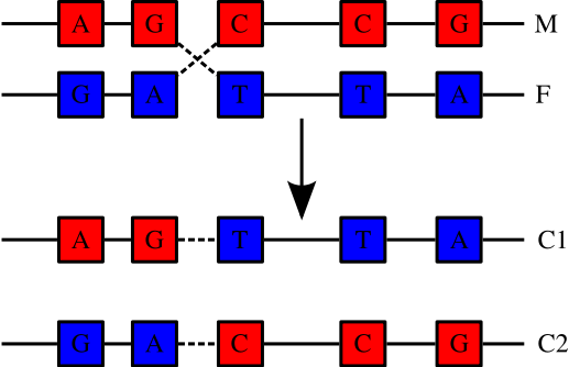
The average number of crossovers per new chromosome is something like 1 per generation. Whereas mutations may change the effect of genes or regulatory sequences, crossing over increases genetic diversity by creating new combinations of previously existing variants. Loci that are closer together on a chromosome are less likely to be separated by recombination. These are more closely linked. Sections of chromosome that are short enough to not be recombined (or not recombined often) are known as haplotype blocks.
Linked loci are likely to show statistical correlation. Linkage equilibrium means that enough recombination has occurred to break up any such correlation. Therefore linkage is often described, confusingly, as Linkage Disequilibrium or LD.
Phylogenetics
Each time a mutation occurs on a haplotype block it creates a slightly different allele or haplotype (although nomenclature can be confusing – sometimes these words are used to describe groups of very similar variants instead) from an existing one.
If we assume that the same mutation doesn’t happen twice then we can trace which allele came from which, and reconstruct a phylogenetic tree. This assumption is known as the infinite sites model: if there were infinite sites where a mutation could happen, the chance of the same mutation happening is zero. In practice, some mutations occur more than once, and to further complicate things, it is not always clear where the boundaries of haplotype blocks are, which means the reconstructions must be done carefully.
Evolutionary model assumes that all species, all individual, and even all haplotype blocks at a given locus, derive from a single ancestor. Intelligent Design allows for the possibility that multiple species, multiple individuals, and multiple genetic variants are primordial; they were designed and then created at a particular point of origin (kind of like the Big Bang in cosmology). If the human race descended from a single couple, and each had two of each kind of chromosome, then there could be up to four primordial haplotype blocks at each loci. Each of these could generate alleles separately.
Evolutionary theorists do not consider this possibility, so if they looked at the same data, they would imagine that the differences between the four haplotype groups must be explained by ancient mutations and a single, much more ancient, phylogenetic tree.
Recombination and Linkage
Humans are diploid (2 sets of chromosomes). We have 46 chromosomes = 22 pairs of autosomes + X + Y . One from each pair comes from each parent. The two chromosomes of each parent may recombine or cross over to create a new chromosome for the child.

The average number of crossovers per new chromosome is something like 1 per generation. Whereas mutations may change the effect of genes or regulatory sequences, crossing over increases genetic diversity by creating new combinations of previously existing variants. Loci that are closer together on a chromosome are less likely to be separated by recombination. These are more closely linked. Sections of chromosome that are short enough to not be recombined (or not recombined often) are known as haplotype blocks.

Linked loci are likely to show statistical correlation. Linkage equilibrium means that enough recombination has occurred to break up any such correlation. Therefore linkage is often described, confusingly, as Linkage Disequilibrium or LD.
Primordial Diversity
Evolutionary model assumes that all species, all individual, and even all haplotype blocks at a given locus, derive from a single ancestor. Intelligent Design allows for the possibility that multiple species, multiple individuals, and multiple genetic variants are primordial; they were designed and then created at a particular point of origin (kind of like the Big Bang in cosmology). If the human race descended from a single couple, and each had two of each kind of chromosome, then there could be up to four primordial haplotype blocks at each locus. Each of these could generate alleles separately.

Evolutionary theorists do not consider this possibility, so if they looked at the same data, they would imagine that the differences between the four haplotype groups must be explained by ancient mutations and a single, much more ancient, phylogenetic tree.
